2. The Duffing Oscillator

In this notebook we will explore the Duffing Oscillator and attempt to recreate the time traces and phase portraits shown on the Duffing Oscillator Wikipedia page

%matplotlib inline
from matplotlib import pyplot as plt

import desolver as de
import numpy as np
from scipy.integrate import solve_ivp

Using `autoray` backend

2.1. Specifying the Dynamical System

Now let’s specify the right hand side of our dynamical system. It should be

\[\ddot x + \delta\dot x + \alpha x + \beta x^3 = \gamma\cos(\omega t)\]

But desolver only works with first order differential equations, thus we must cast this into a first order system before we can solve it. Thus we obtain the following system

\[\begin{split}\begin{array}{l} \frac{\mathrm{d}x}{\mathrm{dt}} = v_x \\ \frac{\mathrm{d}v_x}{\mathrm{dt}} = -\delta v_x - \alpha x - \beta x^3 + \gamma\cos(\omega t) \end{array}\end{split}\]

@de.rhs_prettifier(
    equ_repr="[vx, -𝛿*vx - α*x - β*x**3 + γ*cos(ω*t)]",
    md_repr=r"""
$$
\begin{array}{l}
\frac{\mathrm{d}x}{\mathrm{dt}} = v_x \\
\frac{\mathrm{d}v_x}{\mathrm{dt}} = -\delta v_x - \alpha x - \beta x^3 + \gamma\cos(\omega t)
\end{array}
$$
"""
)
def rhs(t, state, delta, alpha, beta, gamma, omega, **kwargs):
    x,vx = state
    return np.stack([
        vx,
        -delta*vx - alpha*x - beta*x**3 + gamma*np.cos(omega*t)
    ])

print(rhs)
display(rhs)

$$
\begin{array}{l}
\frac{\mathrm{d}x}{\mathrm{dt}} = v_x \\
\frac{\mathrm{d}v_x}{\mathrm{dt}} = -\delta v_x - \alpha x - \beta x^3 + \gamma\cos(\omega t)
\end{array}
$$

\[\begin{split}\begin{array}{l} \frac{\mathrm{d}x}{\mathrm{dt}} = v_x \\ \frac{\mathrm{d}v_x}{\mathrm{dt}} = -\delta v_x - \alpha x - \beta x^3 + \gamma\cos(\omega t) \end{array}\end{split}\]

Let’s specify the initial conditions as well

y_init = np.array([1., 0.])

And now we’re ready to integrate!

2.2. The Numerical Integration

We will use the same constants from Wikipedia as our constants where the forcing amplitude increases and all the other parameters stay constants.

#Let's define the fixed constants

constants = dict(
    delta = 0.3,
    omega = 1.2,
    alpha = -1.0,
    beta  = 1.0,
    gamma = 0.0
)

# The period of the system
T = 2*np.pi / constants['omega']

# Initial and Final integration times
t0 = 0.0
tf = 40 * T

a = de.OdeSystem(rhs, y0=y_init, dense_output=True, t=(t0, tf), dt=0.0001, rtol=1e-14, atol=1e-14, constants={**constants})
a.method = "RK87"

a.reset()
a.constants['gamma'] = 0.2
a.integrate()

2.3. Plotting the State and Phase Portrait

# Times to evaluate the system at
eval_times = np.linspace(18.1, 38.2, 1000)*T

from matplotlib import gridspec

fig = plt.figure(figsize=(20, 4))

gs  = gridspec.GridSpec(1, 2, width_ratios=[3, 1])
ax0 = fig.add_subplot(gs[0])
ax1 = fig.add_subplot(gs[1])
ax1.set_aspect(1)

ax0.plot(eval_times/T, a.sol(eval_times)[:, 0])
ax0.set_xlim(18.1, 38.2)
ax0.set_ylim(0, 1.4)
ax0.set_xlabel(r"$t/T$")
ax0.set_ylabel(r"$x$")
ax0.set_title(r"$\gamma={}$".format(a.constants['gamma']))

ax1.plot(a[18*T:].y[:, 0], a[18*T:].y[:, 1])
ax1.scatter(a[18*T:].y[-1:, 0], a[18*T:].y[-1:, 1], c='red', s=25, zorder=10)
ax1.set_xlim(-1.6, 1.6)
ax1.set_ylim(-1.6, 1.6)
ax1.set_xlabel(r"$x$")
ax1.set_ylabel(r"$\dot x$")
ax1.grid(which='major')
plt.tight_layout()

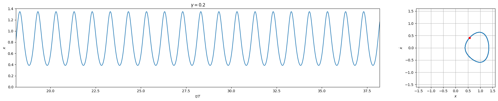
We can see that this plot looks near identical to this plot.

\[\gamma=0.20\]

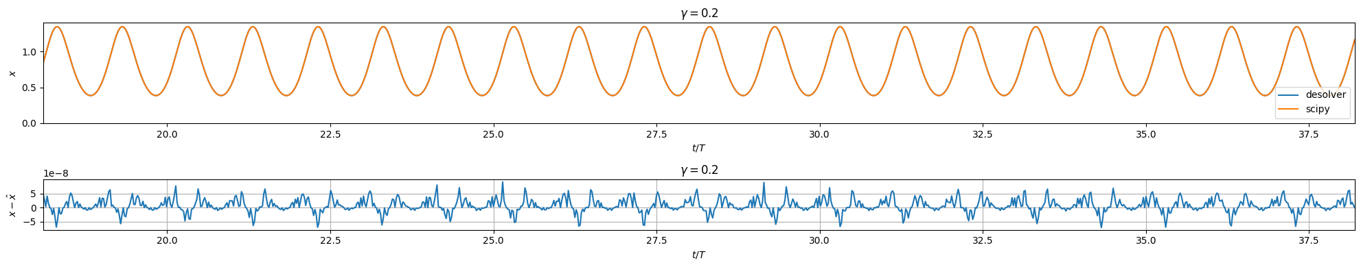
Let’s compare our solution to the solution from scipy.integrate.solve_ivp.

scipy_res = solve_ivp(lambda t, y: rhs(t, y, **a.constants), [t0, tf], y_init, method='LSODA', vectorized=True, rtol=a.rtol, atol=a.atol, dense_output=True)

/home/vscode/.local/share/hatch/env/virtual/desolver/Eduj4EGQ/dev/lib/python3.12/site-packages/scipy/integrate/_ivp/ivp.py:621: UserWarning: At least one element of `rtol` is too small. Setting `rtol = np.maximum(rtol, 2.220446049250313e-14)`.
  solver = method(fun, t0, y0, tf, vectorized=vectorized, **options)

fig = plt.figure(figsize=(20, 4))

gs  = gridspec.GridSpec(2, 1, height_ratios=[2, 1])
ax0 = fig.add_subplot(gs[0])
ax1 = fig.add_subplot(gs[1])

ax0.plot(eval_times/T, a.sol(eval_times)[:, 0], label='desolver')
ax0.plot(eval_times/T, scipy_res.sol(eval_times).T[:, 0], label='scipy')
ax0.set_xlim(18.1, 38.2)
ax0.set_ylim(0, 1.4)
ax0.set_xlabel(r"$t/T$")
ax0.set_ylabel(r"$x$")
ax0.legend()
ax0.set_title(r"$\gamma={}$".format(a.constants['gamma']))

ax1.plot(eval_times/T, a.sol(eval_times)[:, 0] - scipy_res.sol(eval_times).T[:, 0])
ax1.set_xlim(18.1, 38.2)
ax1.set_xlabel(r"$t/T$")
ax1.set_ylabel(r"$x-\hat{x}$")
ax1.set_title(r"$\gamma={}$".format(a.constants['gamma']))
ax1.grid(which='major')
plt.tight_layout()

2.4. Integrating for Different Values of Gamma

Now let’s try to recreate the other plots with the varying gamma values.

gamma_values = [0.28, 0.29, 0.37, 0.5, 0.65]
integration_results = []
integration_results_scipy = []

for gamma in gamma_values:
    a.reset()
    a.constants['gamma'] = gamma

    if gamma == 0.5:
        a.tf = 80.*T
        eval_times = np.linspace(18.1, 78.2, 3000)*T
        integer_period_multiples = np.arange(19, 78)*T
    else:
        a.tf = 40.*T
        eval_times = np.linspace(18.1, 38.2, 1000)*T
        integer_period_multiples = np.arange(19, 38)*T

    a.integrate()
    integration_results.append(((eval_times, a.sol(eval_times)), a.sol(integer_period_multiples)))
    scipy_res = solve_ivp(lambda t, y: rhs(t, y, **a.constants), [t0, tf], y_init, method='LSODA', vectorized=True, rtol=a.rtol, atol=a.atol, dense_output=True)
    integration_results_scipy.append(((eval_times, scipy_res.sol(eval_times).T), scipy_res.sol(integer_period_multiples).T))

for gamma, ((state_times, states), period_states) in zip(gamma_values, integration_results):
    fig = plt.figure(figsize=(20, 4))

    gs  = gridspec.GridSpec(1, 2, width_ratios=[3, 1])
    ax0 = fig.add_subplot(gs[0])
    ax1 = fig.add_subplot(gs[1])
    ax1.set_aspect(1)

    ax0.plot(state_times/T, states[:, 0], zorder=9)
    ax0.set_xlim(state_times[0]/T, state_times[-1]/T)
    if gamma < 0.37:
        ax0.set_ylim(0, 1.4)
    else:
        ax0.set_ylim(-1.6, 1.6)
        ax0.axhline(0, color='k', linewidth=0.5)
    ax0.set_xlabel(r"$t/T$")
    ax0.set_ylabel(r"$x$")
    ax0.set_title(r"$\gamma={}$".format(gamma))

    ax1.plot(states[:, 0], states[:, 1])
    ax1.scatter(period_states[:, 0], period_states[:, 1], c='red', s=25, zorder=10)
    ax1.set_xlim(-1.6, 1.6)
    ax1.set_ylim(-1.6, 1.6)
    ax1.set_xlabel(r"$x$")
    ax1.set_ylabel(r"$\dot x$")
    ax1.grid(which='major')
    plt.tight_layout()

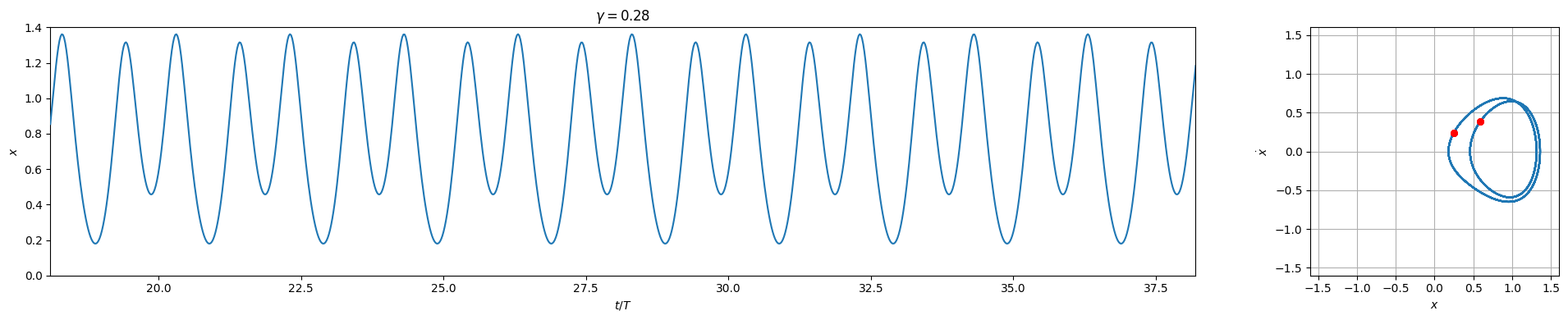
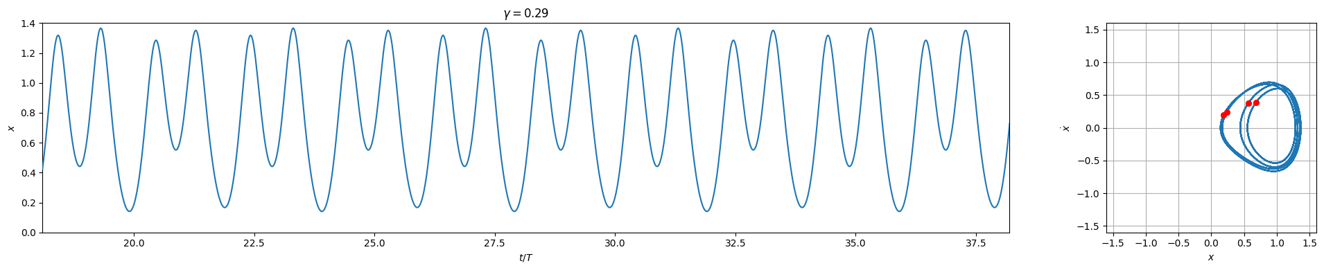
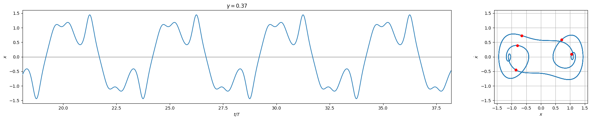
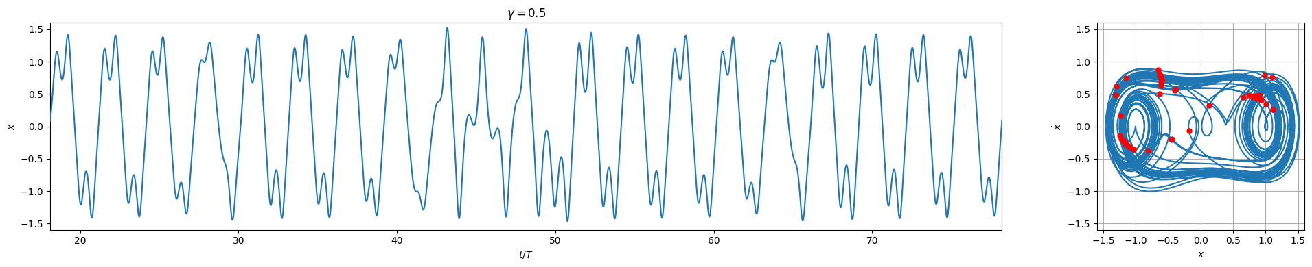
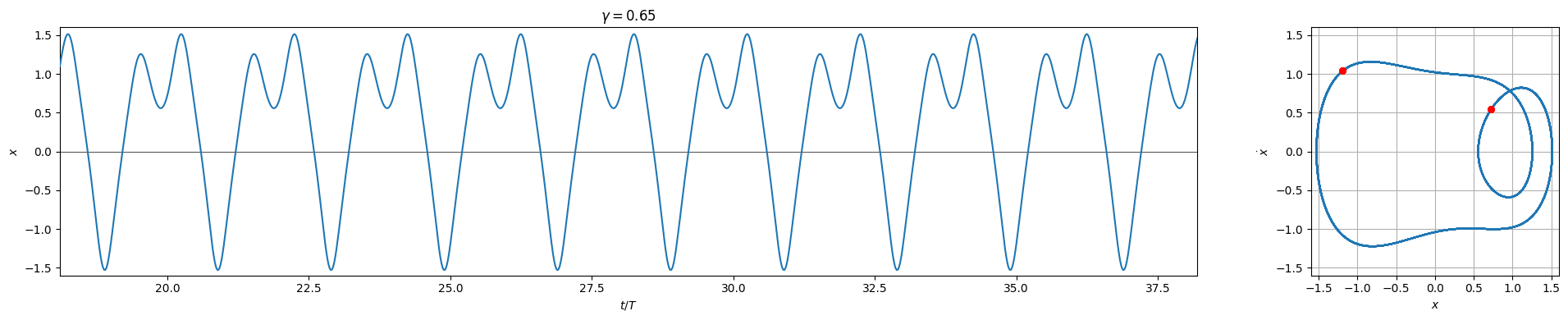
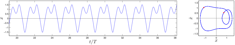
And we see that these plots replicate those on Wikipedia very nicely except for the chaotic one which is highly sensitive to the numerical integrator and tolerances.

( link to image ) \(\gamma = 0.28\)

( link to image ) \(\gamma = 0.29\)

( link to image ) \(\gamma = 0.37\)

( link to image ) \(\gamma = 0.50\)

( link to image ) \(\gamma = 0.65\)

Comparing to solve_ivp we see that, except for the chaotic configurations, the trajectories match very closely.

for gamma, ((state_times, states), period_states), ((state_times_scipy, states_scipy), period_states_scipy) in zip(gamma_values, integration_results, integration_results_scipy):
    fig = plt.figure(figsize=(20, 4))

    gs  = gridspec.GridSpec(2, 2, width_ratios=[3, 1], height_ratios=[2, 1])
    ax0 = fig.add_subplot(gs[0, 0])
    ax1 = fig.add_subplot(gs[0, 1])
    ax2 = fig.add_subplot(gs[1, :])
    ax1.set_aspect(1)

    ax0.plot(state_times/T, states[:, 0], zorder=9, label="desolver")
    ax0.plot(state_times_scipy/T, states_scipy[:, 0], zorder=9, label="scipy")
    ax0.set_xlim(state_times[0]/T, state_times[-1]/T)
    if gamma < 0.37:
        ax0.set_ylim(0, 1.4)
    else:
        ax0.set_ylim(-1.6, 1.6)
        ax0.axhline(0, color='k', linewidth=0.5)
    ax0.set_xlabel(r"$t/T$")
    ax0.set_ylabel(r"$x$")
    ax0.set_title(r"$\gamma={}$".format(gamma))
    ax0.legend()

    ax1.plot(states[:, 0], states[:, 1])
    ax1.scatter(period_states[:, 0], period_states[:, 1], c='red', s=25, zorder=10)
    ax1.set_xlim(-1.6, 1.6)
    ax1.set_ylim(-1.6, 1.6)
    ax1.set_xlabel(r"$x$")
    ax1.set_ylabel(r"$\dot x$")
    ax1.grid(which='major')


    ax2.plot(state_times/T, states[:, 0] - states_scipy[:, 0])
    ax2.set_xlim(18.1, 38.2)
    ax2.set_xlabel(r"$t/T$")
    ax2.set_ylabel(r"$x-\hat{x}$")
    ax2.set_title(r"$\gamma={}$".format(a.constants['gamma']))
    ax2.grid(which='major')
    plt.tight_layout()

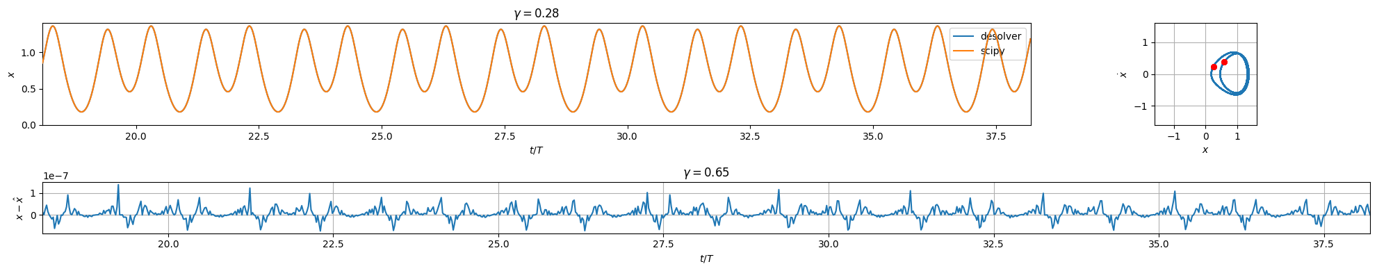
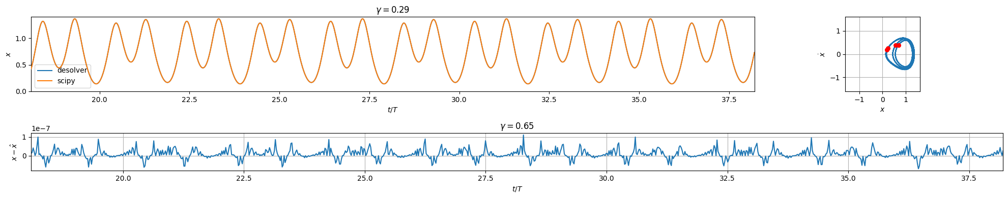
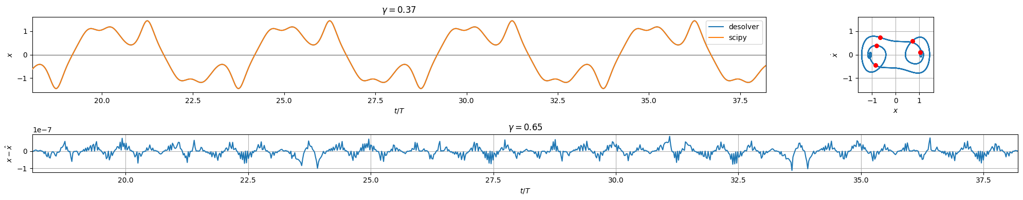
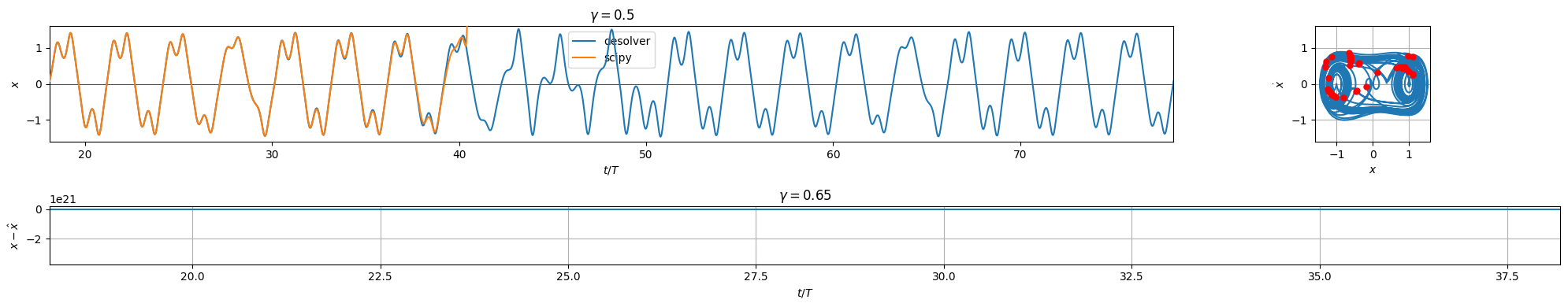
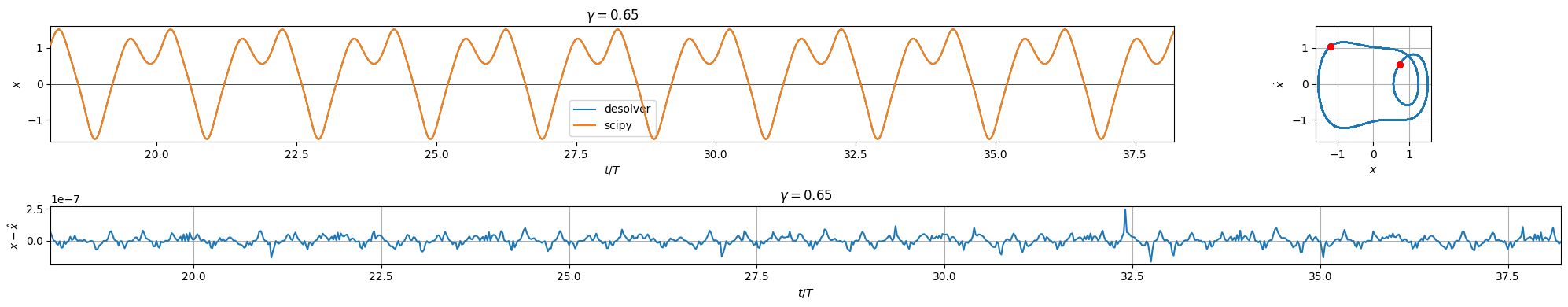
All the solutions, except for the chaotic one at \(\gamma=0.5\), match the solution from solve_ivp. Despite using a method that is generally very effective due to its stiffness detection and method switching, the LSODA method of solve_ivp diverges for the chaotic configuration and takes longer to run.